Deep Learning

How Neural Networks Understand Text, Part 2: LSTM and GRU

How LSTMs use a cell state and gates to control information flow, and how GRU simplifies recurrent networks.

Sai SrinivasOct 29, 20265 min read

In this article

Imagine reading a movie review that says, "The movie is beautiful, despite its slow beginning." To understand the praise, you need to connect "beautiful" with the qualification that follows it. A model reading the sentence one word at a time has to carry useful context forward as each new word arrives.

In Part 1, we saw how a recurrent neural network (RNN) processes text this way, moving through a sequence of timesteps. But standard RNNs can struggle to preserve context across long sequences. During training, vanishing gradients can make distant relationships hard to learn, while exploding gradients can make optimization unstable (Pascanu et al., 2013).

Long short-term memory networks (LSTMs) were designed to help recurrent networks learn long-range dependencies by providing a cell state that can carry information and error signals across many timesteps. Their gates regulate what is retained and updated. This helps with vanishing gradients, but does not make exploding gradients impossible. Hochreiter and Schmidhuber's original LSTM paper.

Rather than maintaining a single state, an LSTM carries two states through the sequence:

Cell state: carries longer-term information and is updated at each timestep.
Hidden state: represents the current output and is passed to the next timestep.

The gates in an LSTM regulate how information enters, remains in, and leaves the cell state.

LSTM Architecture

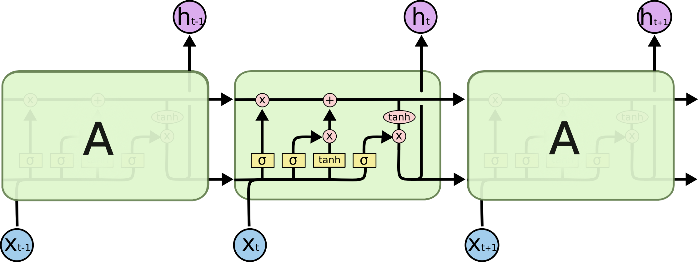
Anatomy of an LSTM Cell

An LSTM cell uses three gates:

Forget gate
Input gate
Output gate

The equations below use $x_t$ for the input at the current timestep, $h_{t-1}$ for the previous hidden state, and $C_{t-1}$ for the previous cell state. The symbol $\odot$ denotes element-wise multiplication.

Forget Gate

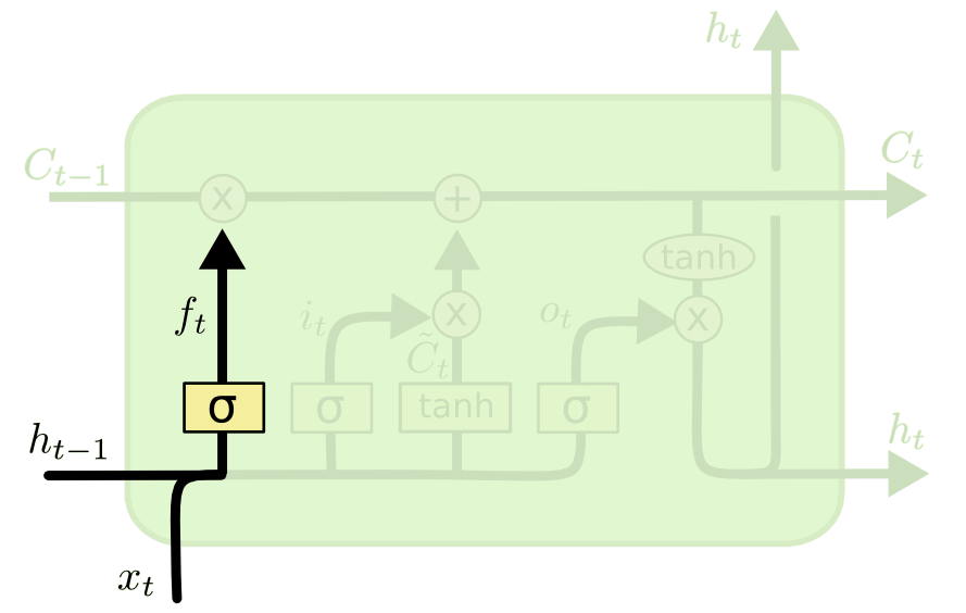
Diagram highlighting the forget gate in an LSTM cell

The forget gate decides which parts of the previous cell state to retain. It combines the current input with the previous hidden state, then applies a sigmoid function to produce values between 0 and 1. Values near 0 suppress information, while values near 1 preserve it.

f_t = \sigma(W_f [h_{t-1}, x_t] + b_f)

C_t^{\mathrm{retained}} = f_t \odot C_{t-1}

The gate does not remove information by itself. Instead, its output scales each component of the previous cell state. Components multiplied by values near zero contribute less to the updated state.

Input Gate

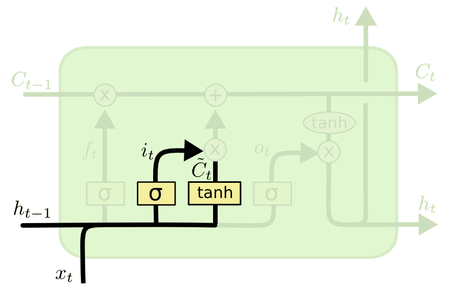
Diagram highlighting the input gate in an LSTM cell

The input gate controls which new information is added to the cell state. First, the cell creates a candidate state. Then the input gate determines how much of each candidate value to use:

\tilde{C}_t = \tanh(W_C [h_{t-1}, x_t] + b_C)

i_t = \sigma(W_i [h_{t-1}, x_t] + b_i)

C_t = f_t \odot C_{t-1} + i_t \odot \tilde{C}_t

Here, $\tilde{C}_t$ is the candidate cell state and $i_t$ is the input gate output. The updated cell state combines retained information with the selected candidate information.

Output Gate

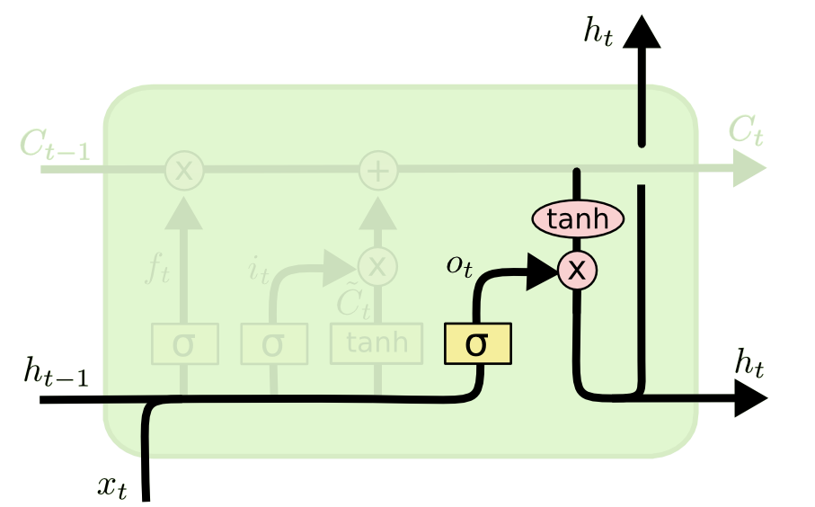
Diagram highlighting the output gate in an LSTM cell

The output gate determines which parts of the updated cell state become the hidden state for the current timestep:

o_t = \sigma(W_o [h_{t-1}, x_t] + b_o)

h_t = o_t \odot \tanh(C_t)

The hidden state $h_t$ is the cell's output. It is passed forward to the next timestep and can also be used by later layers or a prediction head.

Gated Recurrent Units

LSTMs can model long-range relationships, but their multiple gates and two state vectors add parameters and computation. A gated recurrent unit (GRU) is a related architecture that uses a simpler design. In experiments on music and speech sequence modeling, GRUs performed comparably to LSTMs. Results can differ across datasets and model configurations (Chung et al., 2014).

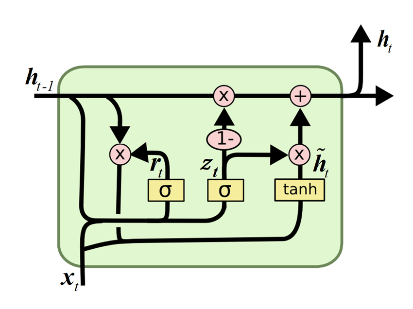
Unlike an LSTM, a GRU maintains one hidden state. Its two gates are the reset gate and the update gate. The diagram below shows the basic GRU architecture.

Diagram showing the basic structure of a gated recurrent unit (GRU) cell

Reset Gate

The reset gate controls how much of the previous hidden state contributes when forming a candidate state:

r_t = \sigma(W_r [h_{t-1}, x_t] + b_r)

Update Gate and Candidate State

The candidate hidden state uses the reset gate to filter the previous hidden state:

\tilde{h}_t = \tanh(W_h [r_t \odot h_{t-1}, x_t] + b_h)

z_t = \sigma(W_z [h_{t-1}, x_t] + b_z)

h_t = (1-z_t) \odot h_{t-1} + z_t \odot \tilde{h}_t

The update gate $z_t$ balances the previous hidden state with the candidate state. This gives the GRU a way to retain useful context while incorporating new information.

References

Long Short-Term Memory by Sepp Hochreiter and Jürgen Schmidhuber
On the Difficulty of Training Recurrent Neural Networks by Razvan Pascanu, Tomas Mikolov, and Yoshua Bengio
Empirical Evaluation of Gated Recurrent Neural Networks on Sequence Modeling by Junyoung Chung, Çaglar Gülçehre, KyungHyun Cho, and Yoshua Bengio
Understanding LSTM: A Deep Dive into Its Inner Workings
Understanding LSTMs by Christopher Olah
The basic structure of a GRU cell
CampusX Deep Learning Playlist